Blog

RNN Neural Network — A Friendly, Informative Guide

admin2 weeks ago

0 23 5 minutes read

RNN Neural Network — A Friendly, Informative Guide

Introduction

Recurrent Neural Networks (RNNs) are a family of neural networks designed to work with sequences data where order matters. If you’ve ever asked your phone to predict the next word, used a speech-to-text app, or seen subtitles auto-generated, there’s a good chance an RNN-style model helped behind the scenes. This article explains what RNNs are, how they work, common variants (LSTM, GRU), training, strengths, weaknesses, and practical tips written clearly so you can understand the ideas and use them.

What is an RNN?

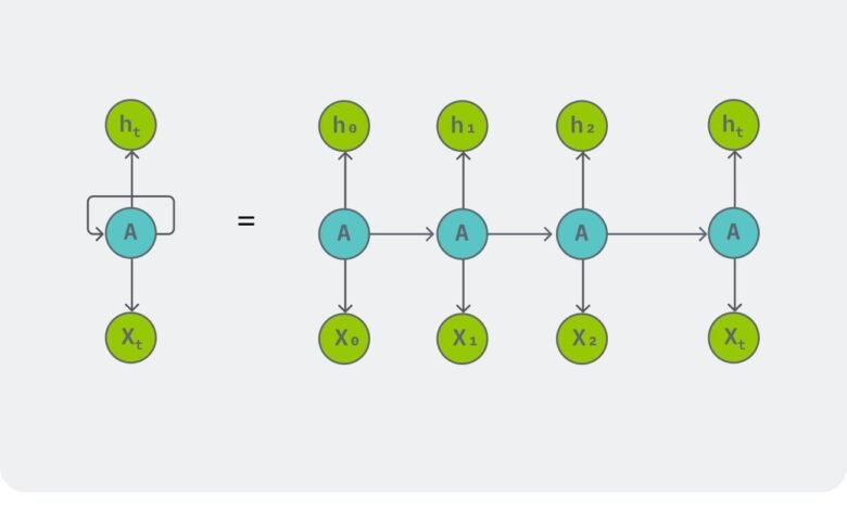
An RNN (Recurrent Neural Network) is a network that processes a sequence one element at a time while keeping a “memory” of previous elements. Unlike feedforward networks that treat every input independently, an RNN has loops inside its architecture that allow information to persist across steps. This makes RNNs well suited to time series, language, audio, and any ordered data.

Example sequence tasks:

Language modeling (predict next word)
Machine translation (sentence → sentence)
Sentiment analysis on text
Time-series forecasting (stock prices, sensor readings)
Speech recognition and generation

The core idea: hidden state and recurrence

At each time step t, an RNN receives an input vector xₜ and updates a hidden state hₜ using both xₜ and the previous hidden state hₜ₋₁. The hidden state is the network’s memory.

A simple mathematical view (vanilla RNN):

W_x and W_h are weight matrices.
activation is typically tanh or ReLU.
y_t is the output at time t (optional for each step or only at the end).

Because the same weights are used at every time step, RNNs have parameter sharing across time, which helps generalize across sequence lengths.

Training RNNs: Backpropagation Through Time (BPTT)

RNNs are trained with gradient-based methods like stochastic gradient descent. To compute gradients across time steps, we “unroll” the RNN into a long feedforward network across time and apply backpropagation this method is called Backpropagation Through Time (BPTT).

Key training behaviors:

Gradients can vanish (become extremely small) or explode (grow very large) as they pass through many time steps. This causes vanilla RNNs to struggle with long-range dependencies.
Techniques to address this include gradient clipping (to handle explosion) and architectural changes (to handle vanishing gradients).

LSTM and GRU — solving the long-range problem

LSTM (Long Short-Term Memory)

LSTM is a widely used RNN variant that uses a memory cell and gating mechanisms to allow the network to store, update, and retrieve information over long time spans. An LSTM cell has:

Input gate — controls how much new information enters the cell
Forget gate — controls how much old information to discard
Output gate — controls what to output from the cell

LSTMs handle long-range dependencies much better than vanilla RNNs and are common in language and speech tasks.

GRU (Gated Recurrent Unit)

GRU is a simpler alternative to LSTM with fewer gates:

Update gate — combines input and forget functionality
Reset gate — decides how to combine new input with past memory

GRUs often achieve similar performance to LSTMs with fewer parameters and faster training.

Variants and advanced structures

Bidirectional RNNs: Process the sequence in both forward and backward directions, useful when the whole sequence is available (e.g., text classification).
Stacked RNNs (deep RNNs): Multiple RNN layers stacked to learn hierarchical patterns.
Sequence-to-sequence (Seq2Seq): Encoder-decoder architectures for tasks like machine translation where one sequence maps to another.
Attention mechanisms: Let the model focus on specific parts of the input sequence. Attention combined with RNNs (or replacing RNNs) improves performance significantly for many tasks.

Strengths of RNN neural network models

Naturally fit sequential data: RNNs can maintain context across sequence elements.
Parameter sharing: Same parameters across time steps makes learning efficient.
Flexible outputs: Can produce outputs per time step or a single output for the whole sequence.

Limitations and when to avoid RNNs

Difficulty with long-range dependencies in vanilla RNNs (mitigated by LSTM/GRU).
Computationally sequential: Processing steps one by one can be slower than parallel-friendly architectures.
Transformers: For many modern language tasks, transformer architectures (which use self-attention and allow parallel processing across sequence positions) have largely outperformed RNNs on large-scale problems. Still, RNNs remain useful for certain tasks and resource-constrained settings.Practical tips for using RNNs

Start with GRU or LSTM instead of vanilla RNN for most tasks.
Use bidirectional RNNs when you can access the entire sequence before prediction.
Regularize with dropout between layers and use layer normalization if training is unstable.
Clip gradients to avoid exploding gradients (e.g., clip norm to a fixed value).
Choose sequence length carefully very long sequences can be truncated or processed in chunks with overlapping windows.
Monitor validation loss for overfitting; RNNs can overfit on small datasets.
Consider attention or transformers if your task needs capturing global dependencies and you have computation budget.

Simple example (PyTorch-style pseudocode)

Below is a short conceptual example showing how an LSTM-based classifier could be set up (not full runnable code, but close enough to guide implementation):

import torch

import torch.nn as nn
class LSTMClassifier(nn.Module):

    def __init__(self, input_size, hidden_size, num_layers, num_classes):

        super().__init__()

        self.lstm = nn.LSTM(input_size, hidden_size, num_layers, batch_first=True)

        self.fc = nn.Linear(hidden_size, num_classes)

def forward(self, x): # x shape: (batch, seq_len, input_size) out, (h_n, c_n) = self.lstm(x) # out: (batch, seq_len, hidden_size) last_hidden = out[:, -1, :] # take last time-step logits = self.fc(last_hidden) # classification output return logits

For sequence-to-sequence tasks you’d use separate encoder and decoder LSTMs and possibly attention.

Applications: where RNNs shine

Natural language processing (NLP): language modeling, named entity recognition, part-of-speech tagging, sentiment analysis.
Speech and audio: speech recognition, speaker identification, audio generation.
Time-series forecasting: financial forecasting, energy demand prediction, sensor data analysis.
Anomaly detection in sequences: detecting unusual patterns over time.
Control systems: modeling sequences of actions or states.

When to choose RNNs vs other models

Choose RNNs (LSTM/GRU) when your data is sequential and you need a model that naturally handles time steps especially when sequences are medium length and compute resources are moderate.
Choose transformers when you need to capture complex long-range dependencies and have enough data and compute. Transformers parallelize better and often yield higher performance on large NLP tasks.
Consider hybrid models: RNN encoder plus attention, or RNNs combined with convolutional layers for structured sequential input like audio spectrograms.

Quick glossary

Hidden state (hₜ): internal memory of the RNN at time t.
BPTT: Backpropagation Through Time, training method for RNNs.
Vanishing/exploding gradients: gradient magnitudes shrink or grow across many time steps, harming training.
LSTM/GRU: gated RNN variants that handle long-range dependencies better.
Bidirectional RNN: reads sequences in both directions.
Attention: mechanism that lets models focus on specific parts of the input.

Final thoughts

RNN neural networks are a foundational family of models for sequence data. While newer architectures like transformers have taken the lead for many large-scale language tasks, RNNs (especially LSTM and GRU) remain important tools in a practitioner’s toolbox. They’re simpler to implement for smaller sequence tasks, efficient on lower-resource devices, and conceptually intuitive for sequential problems.